Heston stochastic volatility model - Calibration
Introduction
The model implements the calibration of Heston stochastic volatility model. HVM assumes that volatility is stochastic and mean reverting.
Calibration
Model Inputs
| Input | Description |
|---|---|
| Current spot | Underlying spot value |
| Initial guess - Heston params | Required for Levenberg Marquadt minimization |
| Lower bound | Lower limit constraint |
| Upper bound | Upper limit constraint |
| Minimization Technique | Differential evoution or Levenberg Marquadt |
| Maximum iterations | Maximum number of iterations for minimization |
| Weights | Observation weight - Equal or Vega weighted |
| Observation data table | Observation data - Strike, Time to maturity, Observed prices, Call type & Discount rates |
Numerical verification of the implemenation
To test the implementation of analytic solution for European call options, results from analytical solution were compared against those from Monte Carlo solutions. Following inputs were considered.
Spot: 1, r = 0.03%, time to maturity = 7 years, Initial variance = 0.1, Long term variance = 0.15, kappa = 3, sigma = 0.2, correlation coeffecient = -0.2, dividend yield = 0%, nSimulations for Monte Carlo = 150000 and nSteps = 150.
Results
| Strike | Monte Carlo price | Analytic solution | Abs Error |
|---|---|---|---|
| 0.25 | 0.808070 | 0.808179 | 0.000109 |
| 0.50 | 0.656430 | 0.654749 | 0.001681 |
| 0.75 | 0.541261 | 0.537977 | 0.003284 |
| 1.00 | 0.452703 | 0.454303 | 0.001600 |
| 1.25 | 0.383353 | 0.383914 | 0.000561 |
| 1.50 | 0.328098 | 0.332173 | 0.004075 |
| 1.75 | 0.283396 | 0.286217 | 0.002821 |
Complex logarithms
The implementation is based on the formula recommended by Gatheral in his book on Volatility surface modelling that avoids discontinuities in option prices emerging while taking principal arguments for complex logarithms. The solution was tested for deep in the money, out of the money as well at the money options with maturities ranging from short time (10-15 days) to long term maturities (30 years) to check if discontinuities exist. The prices were found to be consistent with the those from MC simulations throughout.
Minimization technique
The model offers two minimization techniques - Differential evolution (DE) and Levenberg marquadt (LM). QO recommends using DE whenever a good initial guess is not known. This could be the case when modeling the security for the first time. Unlike LM, DE guarantees a global minima given a sufficient number of iterations.
Weights for observations
Equal weighted, vega weighted or inverse price spread (1/[Pbid-Pask]).
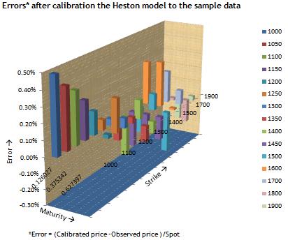
Calibration results
The uploaded model has been pre loaded with sample data. The calibration run on the sample data produced the following results.
Results
| Parameters | DE |
|---|---|
| Initial variance (v0) | 0.190461 |
| Long term variance (theta) | 0.067924 |
| Mean reversion speed (kappa) | 6.237368 |
| Vol of vol (sigma) | 0.920504 |
| Correlation (rho) | -0.755989 |
| RMSE | 3.596383 |
| Time taken(min:sec) | 68:56 |
| Weighted sum of square errors | 65.769942 |
References
- 1. Moodley,Nimalin 2005 "The Heston Model:A Practical Approach"
- 2. Kahl,Christian and Jackel,Peter 2005 "Not-so-complex logarithms in the Heston model"
- 3. Heston, S. (1993). A closed-form solution for options with stochastic volatility. Review of Financial Studies, 6, 327–343.
- 4. Mikhailov,Sergei and Nögel,Ulrich "Heston’s Stochastic Volatility, Model Implementation, Calibration and Some Extensions"